Inertial position

Return to Glossary

Inertial position is the estimated three-dimensional location of a moving body computed exclusively from inertial measurements. An Inertial Navigation System (INS) determines this position by continuously integrating acceleration measurements from an Inertial Measurement Unit (IMU), while compensating for vehicle attitude and Earth’s rotation. Since the computation relies solely on onboard sensors, inertial position remains available in environments where Global Navigation Satellite Systems (GNSS) are unavailable or unreliable.

The estimation process begins with specific force measurements collected by tri-axis accelerometers in the body frame. The INS transforms these measurements into the navigation frame using the attitude matrix $\mathbf{C}_b^n$​, derived from gyroscopes or an Attitude and Heading Reference System (AHRS). Gravity is then restored to recover the true linear acceleration:

$$\mathbf{a}_n = \mathbf{C}_b^n \mathbf{f}_b + \mathbf{g}_n$$

where $\mathbf{f}_b$ is the measured specific force and $\mathbf{g}_n$​ is the local gravity vector.

Velocity is obtained through numerical integration:

$$\mathbf{v}(t)=\mathbf{v}_0+\int_{t_0}^{t}\mathbf{a}_n(\tau)\,d\tau$$

Position follows from a second integration:

$$\mathbf{p}(t)=\mathbf{p}_0+\int_{t_0}^{t}\mathbf{v}(\tau)\,d\tau$$

These mechanization updates execute in real time at sample rates typically ranging from 100 Hz to over 4000 Hz to capture high-frequency vehicle dynamics and minimize numerical integration error.

Accelerometer bias produces velocity errors that increase linearly with time and position errors that grow quadratically.

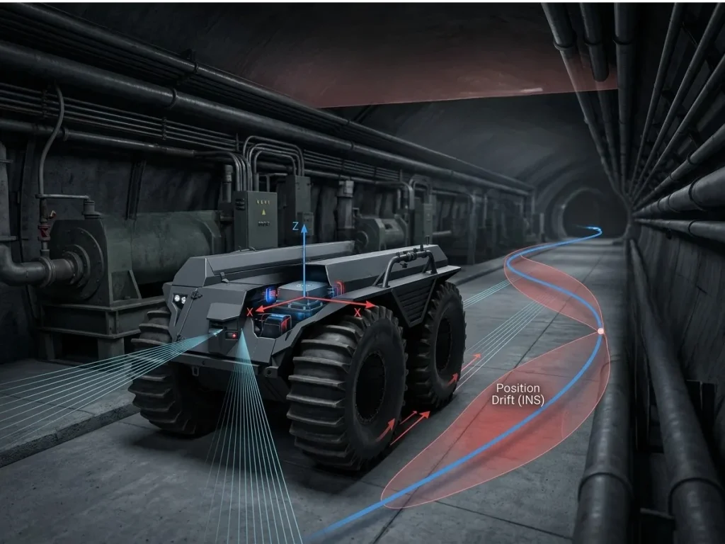
Gyroscope bias introduces attitude errors that misproject gravity, generating additional acceleration errors and accelerating position drift. Consequently, inertial position gradually diverges from the true trajectory during standalone operation.

Position drift

To bound position drift during extended operations, modern navigation systems employ Extended Kalman Filters (EKF), Unscented Kalman Filters (UKF), or pose-graph smoothing algorithms. The filter estimates full-state error vectors (position, velocity, attitude, sensor biases, and scale factors) by fusing high-rate INS mechanization with lower-rate absolute observations from aiding sensors, such as:

• Global Navigation Satellite Systems (GNSS): by using two high-precision correction techniques, RTK and PPP, that reduce that error down to centimeters or even millimeters.
• Acoustic/Speed Sensors: Doppler Velocity Logs (DVL), wheel odometers
• Perceptual Sensors: LiDAR Odometry (LOAM), Visual-Inertial Odometry (VIO)

During GNSS outages, the integrated filter propagates state estimates through INS mechanization in dead-reckoning mode. It uses residual sensor models to constrain error growth until external reference signals return.

High-performance Fiber Optic Gyroscope (FOG), Ring Laser Gyroscope (RLG), and tactical-grade MEMS INS maintain accurate inertial position for extended periods. Inertial position provides a continuous navigation solution by integrating motion dynamics. Its long-term accuracy depends on inertial sensor performance and external aiding measurements.